|
from pylab
import *
# valeurs dans des listes
t =
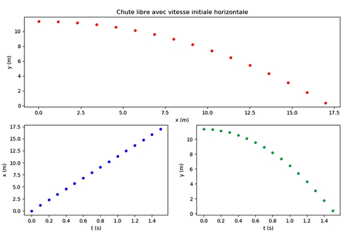
[0, 0.1, 0.2, 0.3, 0.4, 0.5, 0.6, 0.7, 0.8, 0.9]
t += [1, 1.1,
1.2, 1.3, 1.4, 1.5]
x = [0.01, 1.15, 2.3, 3.44, 4.58, 5.72,
6.86, 7.99, 9.12, 10.25]
x += [11.38, 12.52, 13.64, 14.76,
15.88, 16.99]
y = [11.36, 11.31, 11.16, 10.92, 10.57, 10.13,
9.6, 8.96, 8.23, 7.4]
y+=[6.47, 5.44, 4.32, 3.1, 1.79, 0.39]
# graphe 1. Dans un tableau de 2 lignes
et 1 colonne : case 1
subplot(2, 1, 1)
title("Chute
libre avec vitesse initiale horizontale")
scatter(x, y,
s = 18, c = "red", marker =
"o")
xlabel("x
(m)")
ylabel("y (m)")
# graphe 2. Dans un tableau de 2 lignes
et 2 colonnes : case 3
subplot(2, 2, 3)
scatter(t, x,
s = 18, c = "blue", marker =
'o')
xlabel("t (s)")
ylabel("x (m)")
# graphe 3. Dans un tableau de 2 lignes
et 2 colonnes : case 4
subplot(2, 2, 4)
scatter(t, y,
s = 18, c = "#00AA55", marker =
"o")
xlabel("t
(s)")
ylabel("y (m)")
show()
|